Week 1 - Introduction to LLMs and the generative AI project life cycle
Basic definition
- prompt: the input of the model -> the test that you pass into the model
- context window: the space/memory that available to the prompt
- completion: the output of the model
- inference: the act of using the model to generate answers
Base models
Text generation before transformer
It’s important to note that generative algorithms are not new. Previous generations of language models made use of an architecture called recurrent neural networks or RNNs
the limitation of RNN : amount of computation and memory.
An example of RNN carrying out a simple next-word prediction generative task
Why the transformer architecture are powerful?
The power of the transformer architecture lies in its ability to learn the relevance and context of all of the words in a sentence. Not just as you see here, to each word next to its neighbor, but to every other word in a sentence.
Attention weights are apply to those relationships
Attention Map
Self-attention architecture
Self-attention and the ability to learn a tension in this way across the whole input significantly approves the model’s ability to encode language.
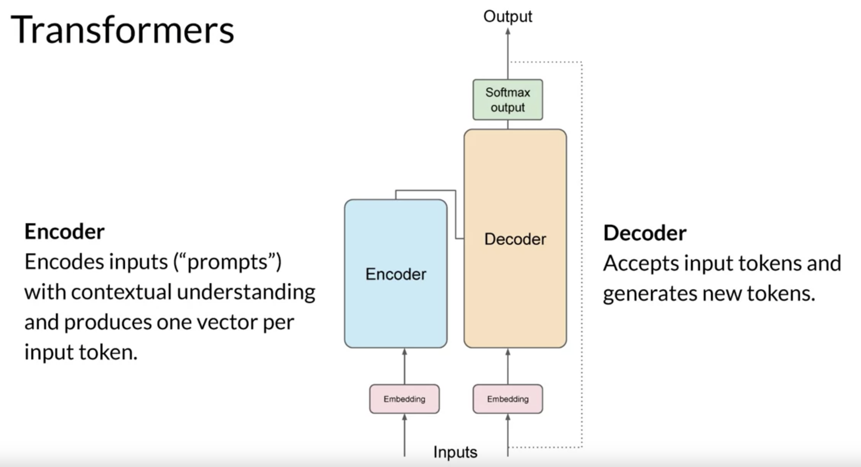
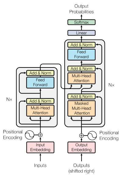
The encoder encodes input sequences into a deep representation of the structure and meaning of the input.
The decoder, working from input token triggers, uses the encoder’s contextual understanding to generate new tokens. It does this in a loop until some stop condition has been reached.
Self-attention Steps
- Tokenize the words
machine-learning models are just big statistical calculators and they work with numbers, not words. So before passing texts into the model to process, you must first tokenize the words.

- numbers passed to the embedding layer
This layer is a trainable vector embedding space, a high-dimensional space where each token is represented as a vector and occupies a unique location within that space. Each token ID in the vocabulary is matched to a multi-dimensional vector, and the intuition is that these vectors learn to encode the meaning and context of individual tokens in the input sequence. Embedding vector spaces have been used in natural language processing for some time, previous generation language algorithms like Word2vec use this concept.
Variants on the basic self-attention model
- Encoder-only models (BERT / T5)
- Decoder-only models (GPT family)
- Encoder-decoder models (BART)
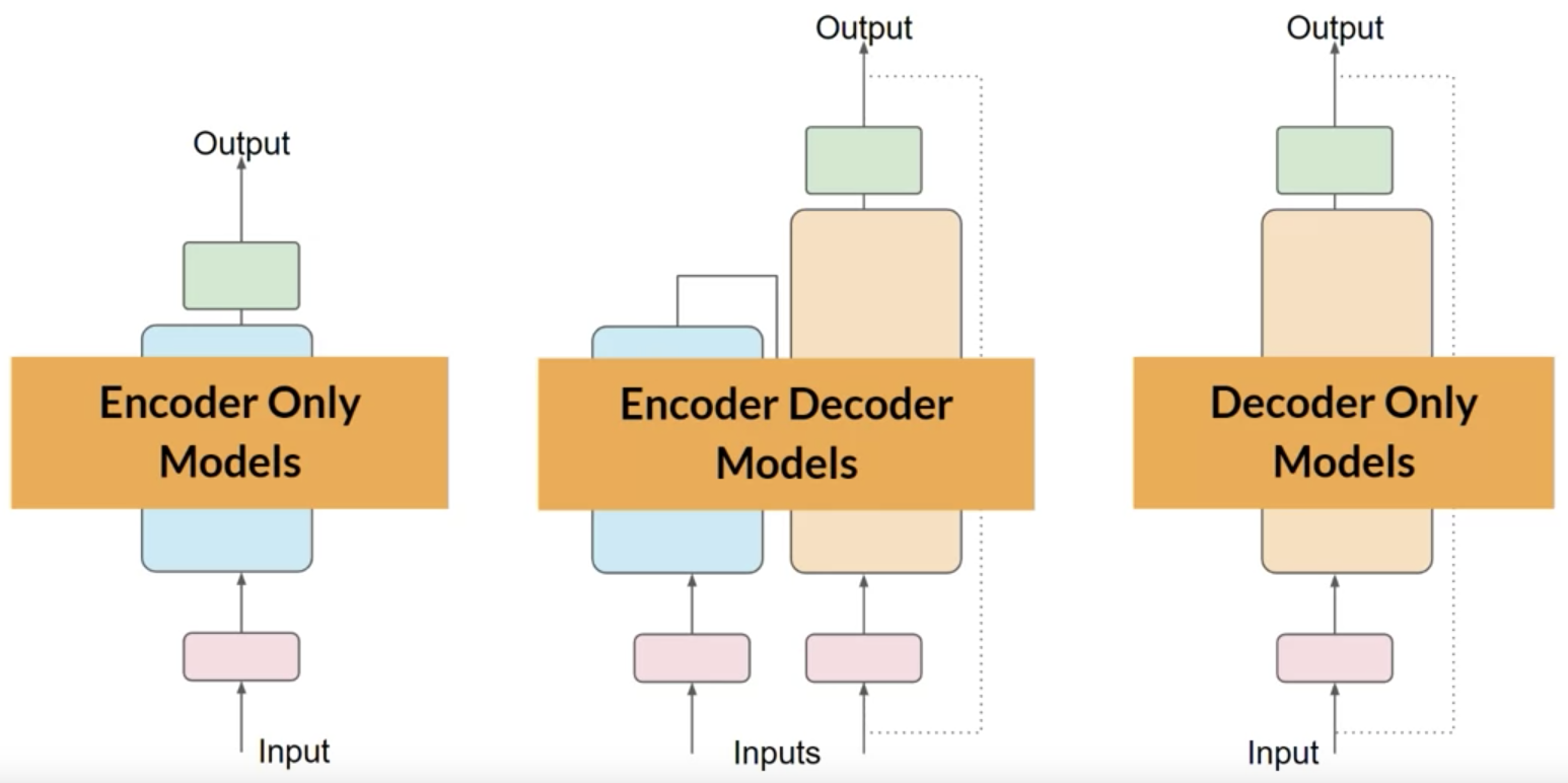
Encoder-only models (BERT / T5)
Also known as Autoencoding models,they are pre-trained using masked language modeling.
Here, tokens in the input sequence or randomly mask, and the training objective is to predict the mask tokens in order to reconstruct the original sentence. This is also called a denoising objective.
Autoencoding models spilled bi-directional representations of the input sequence, meaning that the model has an understanding of the full context of a token and not just of the words that come before. Encoder-only models are ideally suited to task that benefit from this bi-directional contexts.
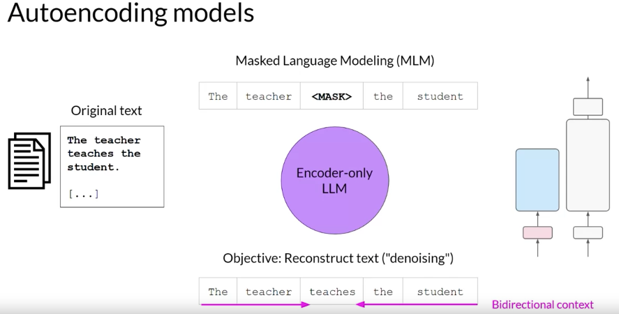
Good to use tasks: ( benefit from bi-directional context)
- Sentiment analysis
- Named entity recognition
- Word classification
eg. BERT and RoBERTa
also work as sequence-to-sequence models, but without further modification, the input sequence and the output sequence or the same length. Their use is less common these days, but by adding additional layers to the architecture, you can train encoder-only models to perform classification tasks such as sentiment analysis. BERT is an example of an encoder-only model.
Decoder-only models (GPT family)
Also known as Autoregressive models,which are pre-trained using causal language modeling.
Here, the training objective is to predict the next token based on the previous sequence of tokens.
Decoder-based autoregressive models, mask the input sequence and can only see the input tokens leading up to the token in question. The model has no knowledge of the end of the sentence. The model then iterates over the input sequence one by one to predict the following token. In contrast to the encoder architecture, this means that the context is unidirectional. By learning to predict the next token from a vast number of examples, the model builds up a statistical representation of language. Models of this type make use of the decoder component off the original architecture without the encoder.
Decoder-only models are often used for text generation, although larger decoder-only models show strong zero-shot inference abilities, and can often perform a range of tasks well. Well known examples of decoder-based autoregressive models are GPT and BLOOM.
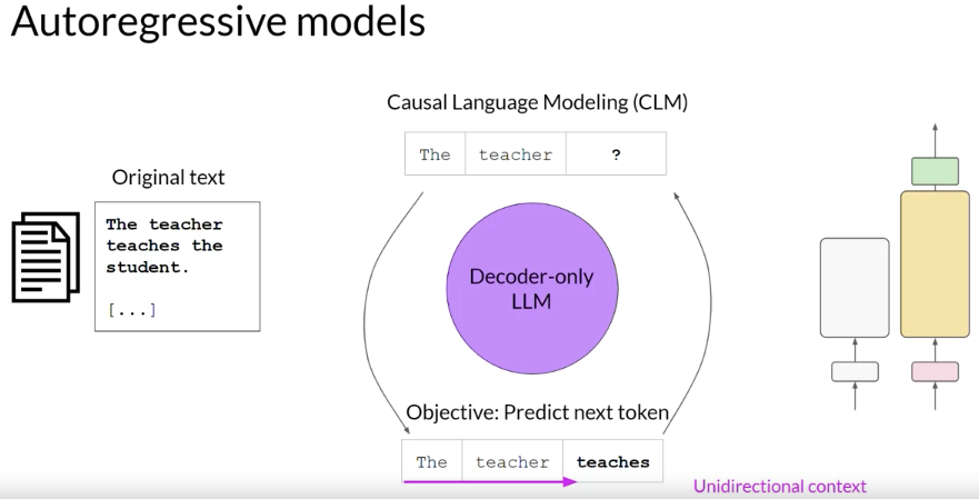
Good to use tasks: ( benefit from bi-directional context)
- Text generation
- Other emergent behavior
eg.GPT and BLOOM
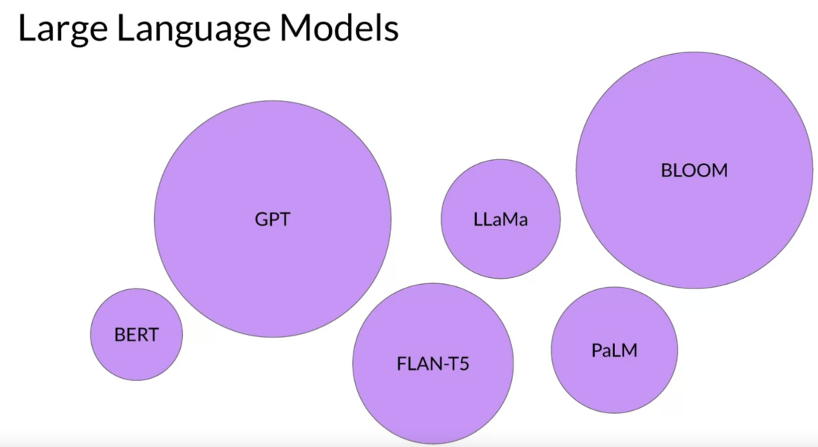
some of the most commonly used today. These models can now generalize to most tasks. Popular decoder-only models include the GPT family of models, BLOOM, Jurassic, LLaMA, and many more.
Encoder-decoder models (T5/ BART)
A popular sequence-to-sequence model T5, pre-trains the encoder using span corruption, which masks random sequences of input tokens. Those mask sequences are then replaced with a unique Sentinel token, shown here as x.
The decoder is then tasked with reconstructing the mask token sequences auto-regressively. The output is the Sentinel token followed by the predicted tokens. You can use sequence-to-sequence models for translation, summarization, and question-answering.
They are generally useful in cases where you have a body of texts as both input and output.
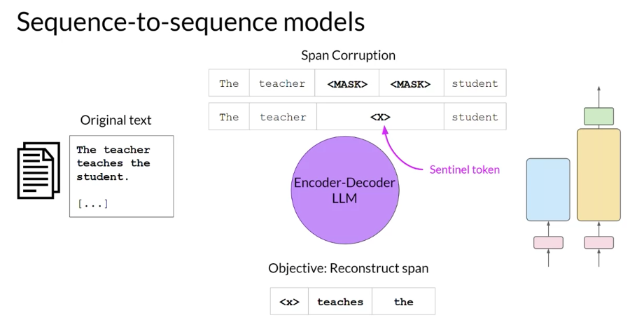
Good to use tasks:
- Translation
- Text summarization
- Question answering
eg.T5 and BART
as you’ve seen, perform well on sequence-to-sequence tasks such as translation, where the input sequence and the output sequence can be different lengths. You can also scale and train this type of model to perform general text generation tasks. Examples of encoder-decoder models include BART as opposed to BERT and T5, the model that you’ll use in the labs in this course.
Summary all architecture
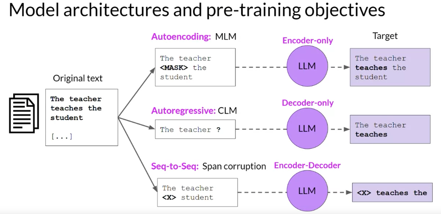
Original paper summary - “Attention is All You Need”
The Transformer architecture consists of an encoder and a decoder, each of which is composed of several layers. Each layer consists of two sub-layers: a multi-head self-attention mechanism and a feed-forward neural network.
- The multi-head self-attention mechanism allows the model to attend to different parts of the input sequence.
- The feed-forward network applies a point-wise fully connected layer to each position separately and identically.
Prompt engineering
-
in-context learning : give examples in prompt
- zero-shot inference

only including your input data within the prompt, is called zero-shot inference. The largest of the LLMs are surprisingly good at this, grasping the task to be completed and returning a good answer.
- one-shot inference
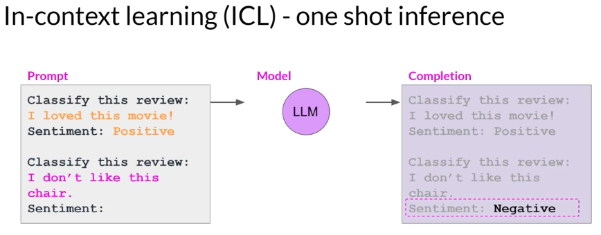
including a single example is known as one-shot inference
- few-shot inference
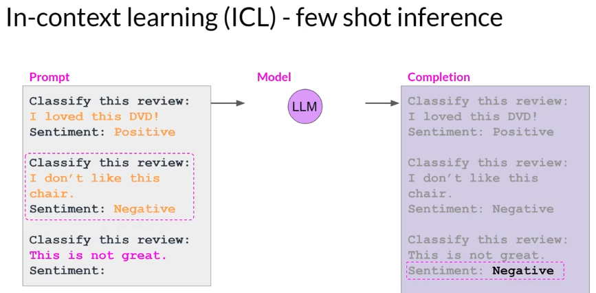
including multiple examples is known as few-shot inference
- zero-shot inference
While the largest models are good at zero-shot inference with no examples, smaller models can benefit from one-shot or few-shot inference that include examples of the desired behavior.
Generative configuration
Configuration parameters
- max new tokens: to limit the number of tokens that the model will generate.
- sample top K: specify the number of tokens to randomly choose from
- sample top P: specify the total probability that you want the model to choose from.
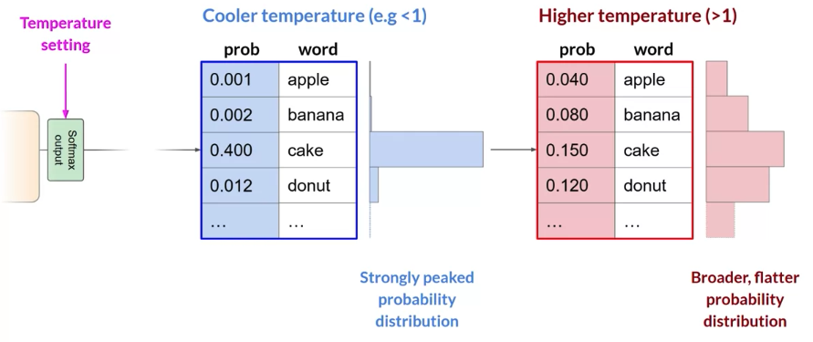
- Temperature: influences the shape of the probability distribution that the model calculates for the next token. Broadly speaking, the higher the temperature, the higher the randomness, and the lower the temperature, the lower the randomness.
Note that these are different than the training parameters which are learned during training time. Instead, these configuration parameters are invoked at inference time and give you control over things like the maximum number of tokens in the completion, and how creative the output is.
The output from the transformer’s softmax layer is a probability distribution across the entire dictionary of words that the model uses.
Greedy decoding V.S. random sampling
greedy : the model will always choose the word with the highest probability; it work very well for short generation but is susceptible to repeated words or repeated sequences of words.
Random sampling is the easiest way to introduce some variability. Instead of selecting the most probable word every time with random sampling, the model chooses an output word at random using the probability distribution to weight the selection.
- sample top K
instructs the model to choose from only the k tokens with the highest probability
- sample top P
setting to limit the random sampling to the predictions whose combined probabilities do not exceed p
Two Settings, top p and top k are sampling techniques that we can use to help limit the random sampling and increase the chance that the output will be sensible.
Temperature setting
Broadly speaking, the higher the temperature, the higher the randomness, and the lower the temperature, the lower the randomness.
Generative AI project lifecycle
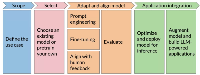
Tips:
getting really specific about what you need your model to do can save you time and perhaps more importantly, compute cost.
Computational challenge to train LLM
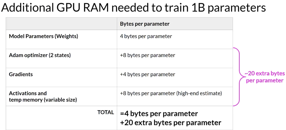
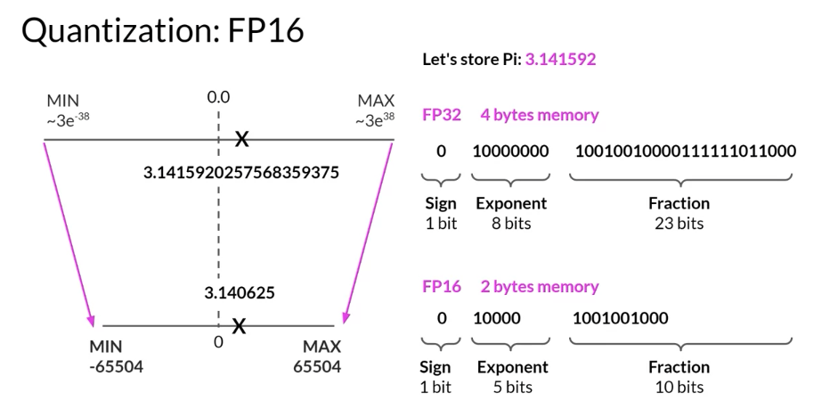
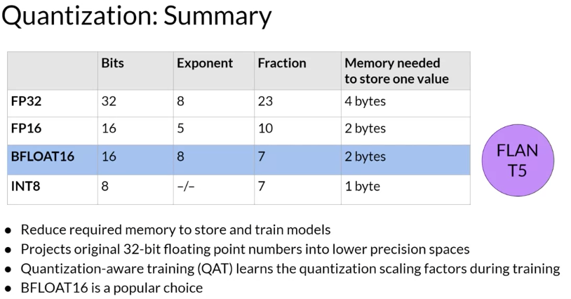
A single parameter is typically represented by a 32-bit float, which is a way computers represent real numbers. You’ll see more details about how numbers gets stored in this format shortly. A 32-bit float takes up four bytes of memory. So to store one billion parameters you’ll need four bytes times one billion parameters, or four gigabyte of GPU RAM at 32-bit full precision.

if only accounted for the memory to store the model weights so far. If you want to train the model, you’ll have to plan for additional components that use GPU memory during training. These include two Adam optimizer states, gradients, activations, and temporary variables needed by your functions.
Solution
Maximize model performance
Remember, the goal during pre-training is to maximize the model’s performance of its learning objective, which is minimizing the loss when predicting tokens.
- scaling dataset size (number of tokens)
- scaling model size (number of parameters)
Distribute Data parallel (DDP)
DDP copyists your model onto each GPU and sends batches of data to each of the GPUs in parallel Note that DDP requires that your model weights and all of the additional parameters, gradients, and optimizer states that are needed for training, fit onto a single GPU.
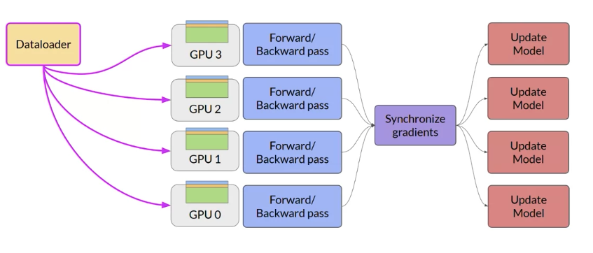
If you model is too big to fit a single GPU, you need use another techniques “model sharding”
- fully sharded data parallel, or FSDP for short
- ZeRO stands for zero redundancy optimizer
the goal of ZeRO is to optimize memory by distributing or sharding model states across GPUs with ZeRO data overlap.
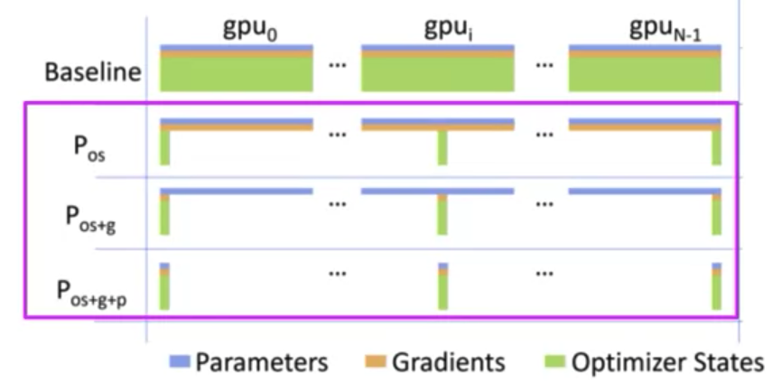
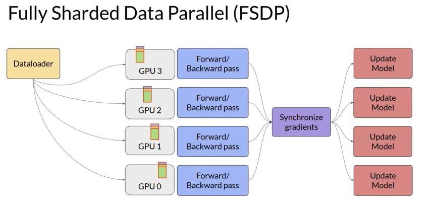
FSDP requires you to collect this data from all of the GPUs before the forward and backward pass.
